The transformer block and the full stack

The whole machine, assembled

Every piece has now been introduced separately. Here they are wired together — drawn with two layers a side rather than six, because the pattern repeats and six of anything is harder to read.

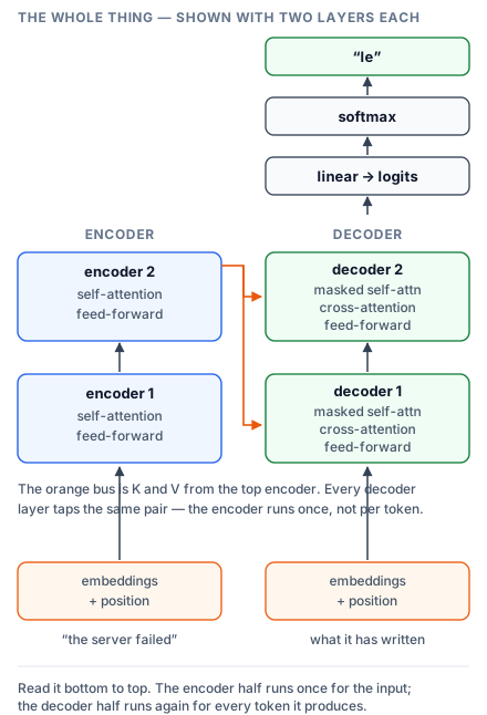
Read it bottom to top. Embeddings plus position enter the bottom of each stack. Each layer hands its output to the layer above. The top decoder's output goes through a linear projection and a softmax to become an actual word.

The orange bus is the part worth slowing down for. The top encoder's output is turned into keys and values once, and every decoder layer taps that same pair. Not each decoder consulting its counterpart encoder — all of them reading from the top of the encoder stack. This is what makes the asymmetry in the picture real: the encoder half runs once per input sentence, the decoder half runs once per output token. Translating a twenty-word sentence means one trip up the encoder and twenty trips up the decoder.

That asymmetry is also the reason a KV cache exists. Since the encoder's keys and values never change while a single output is being generated, recomputing them for every token would be pure waste — so they are computed once and held. The same logic extends to the decoder's own past tokens, which is where the KV cache in the attention course comes from.

Why most models today are half of this picture

The diagram above is the 2017 architecture, built for translation, where there is a clearly separate input to be read and output to be written. Most models you will use are decoder-only: delete the encoder stack, delete the cross-attention sub-layer, and let the single remaining stack read the prompt and continue it as one undifferentiated sequence.

That sounds like a loss and turned out to be a simplification worth making. There is no boundary to decide where input ends and output begins, one stack to scale instead of two, and every task becomes the same task — continue this text. GPT, Llama, Claude and the rest are all this shape. The encoder-decoder form still holds on where input and output really are distinct objects, notably translation and some summarisation.

Read the diagram, then, as the ancestor rather than the current state. The block is unchanged; what changed is how many copies of it there are and whether they are arranged in one stack or two. The next lesson takes that comparison apart properly.

The modern decoder-only transformer block contains two sublayers, each wrapped in a normalization and a residual connection. In the Llama architecture:

h = x + MHA(RMSNorm(x))

output = h + FFN(RMSNorm(h))

That's the complete block. Two sublayers, two norms, two additions. Every architectural innovation in the transformer since 2017 — pre-norm, RMSNorm, RoPE, GQA, SwiGLU — modifies a component within this template, but the template itself hasn't changed. The block is the atom of transformer design: you choose its internals, then stack N copies.

Parameter count for one block (Llama 3 8B)

Llama 3 8B uses $d_{\text{model}} = 4096$, 32 attention heads, 8 key-value heads (grouped-query attention with ratio 4:1), head dimension $d_{h} = 128$, and an FFN intermediate size of 14,336 with SwiGLU activation.

Attention parameters:

• Q projection: d_model × (n_heads × d_h) = 4096 × 4096 = 16,777,216
• K projection: d_model × (n_kv_heads × d_h) = 4096 × (8 × 128) = 4096 × 1024 = 4,194,304
• V projection: d_model × (n_kv_heads × d_h) = 4096 × 1024 = 4,194,304
• O projection: (n_heads × d_h) × d_model = 4096 × 4096 = 16,777,216
• Attention total: 41,943,040 (~42M)

Note: K and V projections are 4x smaller than Q and O because of GQA with 8 KV heads shared across 32 query heads. This saves ~25M parameters per block versus multi-head attention (where K and V would also be 4096 × 4096).

FFN parameters (SwiGLU):

SwiGLU has three weight matrices (no bias):

• Gate projection (W_gate): d_model × d_ff = 4096 × 14,336 = 58,720,256
• Up projection (W_up): d_model × d_ff = 4096 × 14,336 = 58,720,256
• Down projection (W_down): d_ff × d_model = 14,336 × 4096 = 58,720,256
• FFN total: 176,160,768 (~176M)

The FFN dominates: it's 4.2x larger than the attention sublayer. This ratio is typical of modern transformer designs — the intermediate size d_ff is set to 3.5 × d_model (14336/4096 ≈ 3.5), which is the sweet spot found by Llama 2 ablations. The original transformer used $d_{\text{ff}} = 4 \times d_{\text{model}}$, but SwiGLU has three matrices instead of two (a ReLU FFN has only W_1 and W_2), so the intermediate is shrunk to keep total FFN parameters comparable.

Norm parameters:

• 2 × RMSNorm with d_model parameters each = 2 × 4096 = 8,192

Per-block total: 41,943,040 + 176,160,768 + 8,192 = 218,112,000 (~218M)

Full model:

• 32 blocks: 32 × 218,112,000 = 6,979,584,000 (~6.98B)
• Token embedding: vocab_size × d_model = 128,256 × 4096 = 525,336,576 (~525M)
• Final RMSNorm: 4,096
• LM head (untied): d_model × vocab_size = 4096 × 128,256 = 525,336,576 (~525M)
• Grand total: 6,979,584,000 + 525,336,576 + 4,096 + 525,336,576 = 8,030,261,248

This matches Meta's published 8.03B parameter count for Llama 3 8B.

The block in code

import torch
import torch.nn as nn
import torch.nn.functional as F

class RMSNorm(nn.Module):
    def __init__(self, dim, eps=1e-6):
        super().__init__()
        self.weight = nn.Parameter(torch.ones(dim))
        self.eps = eps

    def forward(self, x):
        rms = torch.sqrt(x.pow(2).mean(-1, keepdim=True) + self.eps)
        return x / rms * self.weight


class Attention(nn.Module):
    def __init__(self, d_model, n_heads, n_kv_heads):
        super().__init__()
        self.n_heads = n_heads
        self.n_kv_heads = n_kv_heads
        self.head_dim = d_model // n_heads
        self.n_rep = n_heads // n_kv_heads

        self.wq = nn.Linear(d_model, n_heads * self.head_dim, bias=False)
        self.wk = nn.Linear(d_model, n_kv_heads * self.head_dim, bias=False)
        self.wv = nn.Linear(d_model, n_kv_heads * self.head_dim, bias=False)
        self.wo = nn.Linear(n_heads * self.head_dim, d_model, bias=False)

    def forward(self, x, mask=None):
        B, T, C = x.shape
        q = self.wq(x).view(B, T, self.n_heads, self.head_dim).transpose(1, 2)
        k = self.wk(x).view(B, T, self.n_kv_heads, self.head_dim).transpose(1, 2)
        v = self.wv(x).view(B, T, self.n_kv_heads, self.head_dim).transpose(1, 2)

        if self.n_rep > 1:
            k = k.repeat_interleave(self.n_rep, dim=1)
            v = v.repeat_interleave(self.n_rep, dim=1)

        scale = self.head_dim ** -0.5
        attn = (q @ k.transpose(-2, -1)) * scale
        if mask is not None:
            attn = attn.masked_fill(mask == 0, float("-inf"))
        attn = F.softmax(attn, dim=-1)
        out = (attn @ v).transpose(1, 2).contiguous().view(B, T, -1)
        return self.wo(out)


class SwiGLU_FFN(nn.Module):
    def __init__(self, d_model, d_ff):
        super().__init__()
        self.w_gate = nn.Linear(d_model, d_ff, bias=False)
        self.w_up = nn.Linear(d_model, d_ff, bias=False)
        self.w_down = nn.Linear(d_ff, d_model, bias=False)

    def forward(self, x):
        return self.w_down(F.silu(self.w_gate(x)) * self.w_up(x))


class TransformerBlock(nn.Module):
    def __init__(self, d_model, n_heads, n_kv_heads, d_ff):
        super().__init__()
        self.attn_norm = RMSNorm(d_model)
        self.attn = Attention(d_model, n_heads, n_kv_heads)
        self.ffn_norm = RMSNorm(d_model)
        self.ffn = SwiGLU_FFN(d_model, d_ff)

    def forward(self, x, mask=None):
        h = x + self.attn(self.attn_norm(x), mask)
        out = h + self.ffn(self.ffn_norm(h))
        return out

The full model: embedding to logits

class Transformer(nn.Module):
    def __init__(self, vocab_size, d_model, n_layers, n_heads, n_kv_heads, d_ff):
        super().__init__()
        self.embed = nn.Embedding(vocab_size, d_model)
        self.layers = nn.ModuleList([
            TransformerBlock(d_model, n_heads, n_kv_heads, d_ff)
            for _ in range(n_layers)
        ])
        self.norm = RMSNorm(d_model)
        self.lm_head = nn.Linear(d_model, vocab_size, bias=False)

    def forward(self, input_ids):
        B, T = input_ids.shape
        x = self.embed(input_ids)

        mask = torch.tril(torch.ones(T, T, device=x.device)).unsqueeze(0).unsqueeze(0)
        for layer in self.layers:
            x = layer(x, mask)

        x = self.norm(x)
        logits = self.lm_head(x)  # (B, T, vocab_size)
        return logits


# Instantiate with Llama 3 8B dimensions
model = Transformer(
    vocab_size=128_256,
    d_model=4096,
    n_layers=32,
    n_heads=32,
    n_kv_heads=8,
    d_ff=14_336,
)

total_params = sum(p.numel() for p in model.parameters())
print(f"Total parameters: {total_params:,}")
# Output: Total parameters: 8,030,261,248

End-to-end data flow

The complete forward pass for generating one token:

• Tokenize: BPE segmentation converts raw text into token IDs. "The capital of France is" → [The, capital, of, France, is] → [791, 6864, 315, 9822, 374] (5 tokens with Llama 3's 128K-token vocabulary).
• Embed: lookup each ID in the embedding matrix E of shape (128256, 4096). Result: a tensor of shape (1, 5, 4096) — each token is now a 4096-dimensional vector. No positional encoding is added here (RoPE is applied inside attention, not to the embedding).
• 32 transformer blocks: each applies attention (with RoPE rotations, GQA, causal mask) followed by SwiGLU FFN, both wrapped in pre-norm residual connections. After all 32 blocks, the residual stream has been updated 64 times (32 attention writes + 32 FFN writes).
• Final RMSNorm: normalize the output of the last block to a consistent scale before the linear projection.
• LM head: linear projection from $d_{\text{model}} = 4096$ to vocab_size = 128,256, producing raw logits of shape (1, 5, 128256).
• Sample: take the logits at the last position (128256,), optionally apply temperature scaling (logits / temperature) and top-p nucleus filtering, convert to probabilities via softmax, sample one token ID from the distribution.
• Repeat: append the sampled token to the input and run another forward pass. With KV caching, only the new token's attention computation is performed — all previous tokens' keys and values are reused from cache, making generation cost O(T) per token rather than O(T²).

The language model head and weight tying

The LM head is a linear layer mapping R^d_model → R^vocab_size. Its weight matrix has shape (vocab_size, d_model) — the same shape as the embedding matrix (transposed). Weight tying (Press & Wolf 2017, "Using the Output Embedding to Improve Language Models") sets LM_head.weight = Embedding.weight, reducing parameter count by vocab_size × d_model and providing a regularization benefit: the model is forced to use the same vector space for "reading a token" (embedding lookup) and "predicting a token" (projecting onto the vocabulary).

GPT-2 (Radford et al. 2019) and GPT-3 (Brown et al. 2020) use weight tying. Llama 3 does NOT — it uses a separate, untied LM head. Meta's reasoning: with a 128K vocabulary and $d_{\text{model}} = 4096$, tying forces the embedding to be a rank-4096 matrix of size 128K × 4096. An untied architecture allows the embedding and LM head to learn different specializations — the embedding optimizes for input discrimination (distinguishing between tokens) while the LM head optimizes for output prediction (ranking the correct next token above all others). The 525M parameter cost of a separate LM head is ~6.5% of the total model — a modest cost for the added flexibility.

Depth vs. width: why 32 layers and not 2

A 2-layer model with $d_{\text{model}} = 32768$ has roughly the same parameter count as a 32-layer model with $d_{\text{model}} = 4096$ (the FFN dominates, so parameters scale roughly as L × d_model × d_ff). But they behave very differently.

Kaplan et al. 2020 ("Scaling Laws for Neural Language Models") found that for a fixed parameter budget, increasing depth provides better loss-per-parameter than increasing width — up to a point. Each layer adds one "step" of computation that can compose with all previous steps. A 32-layer model can implement 32-step algorithms — it has 32 opportunities to transform the representation, each conditioned on all prior transformations. A 2-layer model, regardless of width, can only implement 2-step computations.

Concretely: factual recall (Q: "The capital of France is..." A: "Paris") requires at minimum ~3 layers in practice (Geva et al. 2023) — one to identify the query structure, one to retrieve the fact, one to format the output. Multi-hop reasoning (Q: "The birthplace of the inventor of the telephone is..." → Bell → Edinburgh) requires more. Two layers cannot chain these operations.

The flip side: very deep models are harder to train even with residuals. Beyond ~100 layers, training instabilities emerge from accumulated floating-point errors in the residual additions, correlation between layer outputs (later layers' inputs are increasingly determined by early layers), and the optimization landscape becoming increasingly non-convex. Current practice for frontier models: 32 layers (7–8B), 40 layers (13B), 80 layers (70B), and 126 layers (405B, Llama 3.1).

FLOPs per forward pass

For a transformer with L layers, sequence length T, model dimension d, and FFN intermediate dimension d_ff, the dominant operations are matrix multiplications. Counting multiply-accumulate operations (MACs, where 1 MAC = 2 FLOPs):

• Attention projections (Q, K, V, O) per layer: 4 × 2 × T × d² FLOPs for standard MHA (with GQA, K and V are cheaper, but Q and O dominate)
• Attention score computation: 2 × T² × d (QK^T) + 2 × T² × d (score × V) = 4 × T² × d
• FFN (SwiGLU) per layer: 3 × 2 × T × d × d_ff = 6 × T × d × d_ff

For Llama 3 8B (d=4096, d_ff=14336, L=32, T=4096):

• Attention projections per layer: 4 × 2 × 4096 × 4096² ≈ 549G FLOPs (simplified; GQA reduces this by ~20%)
• Attention scores per layer: 4 × 4096² × 4096 ≈ 275G FLOPs
• FFN per layer: 6 × 4096 × 4096 × 14336 ≈ 1,448G FLOPs
• Total per layer: ~2,100G FLOPs
• All 32 layers: ~67.2 TFLOPs per forward pass

The T² term in attention is negligible at T=4096 (275G vs 1,997G from linear terms = ~12% of compute). At T=128K, it would dominate: 4 × 128K² × 4096 ≈ 274T FLOPs per layer just for attention scores — which is why long-context models require architectural modifications (sliding window, ring attention, or approximations) to remain computationally feasible.