Residual connections and the residual stream

Every sub-layer is wrapped the same way

No sub-layer in a transformer is ever wired straight into the next one. Each is wrapped in the same two-part envelope, and the envelope is so uniform it is easy to read past — which is a mistake, because without it the stack does not train at all.

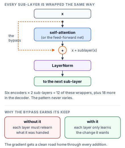
The input x goes two ways. One copy passes through the sub-layer; the other skips it entirely. The two are added, and the sum is normalised. Written out: LayerNorm(x + sublayer(x)).

The addition changes what a layer is for. Without the bypass, each layer must output a complete replacement representation — everything worth keeping has to be reconstructed from scratch, and any layer that fails to reconstruct something destroys it for every layer above. With the bypass, the layer outputs only a correction. It says what to change, and everything it says nothing about passes through untouched. A layer with nothing to contribute can output near-zero and cost nothing, which is a far easier thing for gradient descent to find than an identity function built out of matrix multiplies.

The training argument is the sharper one. The gradient flowing backwards through an addition splits and travels both paths. One goes through the sub-layer and gets multiplied by its Jacobian, shrinking as gradients do. The other takes the bypass and arrives unchanged. Stack 96 layers and the second path still delivers a usable gradient to layer 1 — the deep-network training problem from lesson 1, solved not by making each layer better behaved but by giving the gradient a road that goes around them.

This is why the shape had to stay fixed. x + sublayer(x) is only defined if both are 512 wide, which is what forces every sub-layer in the network to preserve width.

The consequence is a way of seeing the whole architecture that is worth carrying forward. Because every sub-layer only ever adds to a running vector, that vector behaves less like a pipeline and more like a shared channel that each sub-layer reads from and writes to — the residual stream. Attention heads read what earlier layers wrote and add their findings back; feed-forward layers do the same. The stream is the model's working memory, and it is a bus, not a conveyor belt.

Every sublayer in a transformer — every attention mechanism, every feed-forward network — adds its output to its input rather than replacing it. In the pre-norm formulation: output = x + Sublayer(Norm(x)). The + x is the residual connection. Without it, a 32-layer transformer would require information from the embedding layer to survive 64 successive nonlinear transformations (32 attention layers + 32 FFN layers) — each one a potential bottleneck that could corrupt, dilute, or entirely erase the original signal. With residual connections, the input has a guaranteed additive path to the output regardless of what each sublayer computes.

The gradient flow argument

Consider a simplified transformer with L layers, where layer l computes $x_{l} = x_{l - 1} + f_{l}(x_{l - 1})$. The final output is x_L. Taking the derivative of the loss J with respect to an early layer's output x_k:

Expanding ∂x_L/∂x_k by unrolling the recursion $x_{l} = x_{l - 1} + f_{l}(x_{l - 1})$:

The critical term is I — the identity matrix. It guarantees that even if every intermediate Jacobian ∂f_l/∂x has spectral norm less than 1 (meaning the sublayer's transformation is contractive — it shrinks its input), the gradient of the loss with respect to x_k always contains a component exactly equal to ∂J/∂x_L. The gradient at the final layer passes directly back to layer k without any multiplicative attenuation from intervening transformations.

Without residual connections, the gradient becomes a product of Jacobians:

which collapses to:

where g_l is the full layer (no residual). Each Jacobian ∂g_l/∂x_{l-1} is a d_model × d_model matrix. If its spectral norm is consistently less than 1 (contractive), the product shrinks exponentially: for L - k = 30 layers with spectral norm 0.9, the gradient is attenuated by 0.9^30 ≈ 0.04 — a 25x reduction. If the spectral norm exceeds 1 consistently, the gradient grows exponentially — exploding gradients. Getting every layer's Jacobian spectral norm to hover near 1 across all training steps and all input examples is impractical without architectural help. Residual connections provide that help by construction, adding the identity to each layer's effective Jacobian.

This was demonstrated in He et al. 2016 (Deep Residual Learning for Image Recognition) for convolutional networks and has proven equally essential for transformers. Without residual connections, no one has successfully trained a transformer beyond ~12 layers.

What sublayers actually compute under the residual regime

Because each sublayer adds to the running representation rather than overwriting it, the output of the final layer can be decomposed as a sum:

where x_0 is the token embedding and each f_l is either an attention sublayer or an FFN sublayer. The final representation is the embedding plus the sum of all sublayer contributions. This additive structure has a profound consequence: each sublayer's contribution can be studied in isolation. You can measure what each attention head or FFN writes into the representation by computing f_l(x_{l-1}) — it's a vector in R^d_model that was added to the stream. You don't need to disentangle it from a composition of nonlinearities.

Furthermore, if a sublayer produces near-zero output (its contribution has small norm), the input passes through essentially unchanged. This means sublayers can be "active" on some inputs and "inactive" on others — a form of conditional computation that emerges naturally from training. Empirically, late FFN layers in large models often produce very small outputs for common tokens (the model has already computed the correct representation by that point) and large outputs only for difficult or unusual tokens.

The residual stream (Elhage et al. 2021)

Anthropic's "A Mathematical Framework for Transformer Circuits" (Elhage, Neel, et al. 2021) formalizes this additive view by defining the residual stream: the d_model-dimensional vector at each token position, which starts as the token embedding and is incrementally updated by each sublayer as the token passes through the network.

The residual stream acts as a shared memory bus with the following access pattern:

• Each attention head reads from the stream (via Q, K, V projections applied to the stream's current state) and writes back (adding its output projection to the stream). Attention heads can read from one subspace of the stream and write to a completely different subspace.
• Each FFN layer reads from the stream (its input weight matrix selects which directions to attend to) and writes back (its output weight matrix determines which directions to modify).
• The LM head reads from the final stream state to produce logits over the vocabulary.

Because Q, K, V, O projections are all linear transformations, the stream naturally decomposes into subspaces. An attention head at layer 5 might write information into a particular direction in R^d_model — say, "the subject of this sentence is a country." A later FFN at layer 20 might have input weights that project strongly onto exactly that direction, allowing it to read that "country" feature and activate its "capitals knowledge" neurons. Intermediate layers (6 through 19) that don't need this feature leave it untouched — the residual connection preserves it exactly through all those layers.

This enables superposition: the stream has d_model dimensions (e.g., 4096) but the model encodes far more than 4096 independent features by storing them as nearly-orthogonal directions. Anthropic's later work (Bricken et al. 2023, "Towards Monosemanticity") found that a single-layer model with $d_{\text{model}} = 512$ encodes thousands of interpretable features in superposition, and the residual stream is what allows later layers to selectively read the features they need.

Tracing a token through the residual stream

import torch
from transformers import AutoModelForCausalLM, AutoTokenizer

model_name = "meta-llama/Llama-3.2-1B"
tokenizer = AutoTokenizer.from_pretrained(model_name)
model = AutoModelForCausalLM.from_pretrained(
    model_name, torch_dtype=torch.float32, device_map="cpu"
)

text = "The capital of France is"
inputs = tokenizer(text, return_tensors="pt")
input_ids = inputs["input_ids"]

# Use output_hidden_states to get the residual stream at every layer
with torch.no_grad():
    outputs = model(input_ids, output_hidden_states=True)
    hidden_states = outputs.hidden_states
    # hidden_states[0] = embedding output
    # hidden_states[i] = output of layer i (after residual addition)
    # hidden_states[-1] = output of final layer (before final norm)

# Analyze the last token's residual stream evolution
last_token_idx = input_ids.shape[1] - 1
token_text = tokenizer.decode(input_ids[0, last_token_idx])
print(f"Tracking residual stream for token: '{token_text}'")
print(f"Position: {last_token_idx}, Model layers: {len(hidden_states) - 1}")

# Compute per-layer deltas and cosine similarities
print(f"\n{'Layer':<6} {'Delta norm':<12} {'Stream norm':<12} {'Cos(l, l-1)':<12}")
print("-" * 44)
for i in range(1, len(hidden_states)):
    prev = hidden_states[i-1][0, last_token_idx]
    curr = hidden_states[i][0, last_token_idx]
    delta = curr - prev
    delta_norm = delta.norm().item()
    stream_norm = curr.norm().item()
    cos_sim = torch.nn.functional.cosine_similarity(
        curr.unsqueeze(0), prev.unsqueeze(0)
    ).item()
    print(f"{i:<6} {delta_norm:<12.3f} {stream_norm:<12.3f} {cos_sim:<12.4f}")

# What does the model predict from the final hidden state?
logits = outputs.logits[0, last_token_idx]
top5 = torch.topk(logits, 5)
print(f"\nTop 5 predictions after '{text}':")
for score, idx in zip(top5.values, top5.indices):
    print(f"  {tokenizer.decode([idx])!r:>12}: {score.item():.2f}")

Running this on Llama 3.2 1B (16 layers) reveals a characteristic pattern:

• Early layers (1–4): high cosine similarity with the previous layer (~0.99), small delta norms. The sublayers are making fine adjustments to the embedding — primarily learning positional and local syntactic patterns. The stream hasn't moved far from the original embedding.
• Middle layers (5–11): cosine similarity drops (0.95–0.98), delta norms peak. These layers perform the heavy computational work — factual associations (France → Paris), entity resolution, semantic composition. The stream is being steered rapidly toward the correct output direction.
• Late layers (12–16): cosine similarity rises again (~0.98–0.99), delta norms decrease. The model is formatting the output — fine-tuning the representation's projection onto the vocabulary space to sharpen the logit distribution.

The residual stream enables composition across layers

A concrete example of cross-layer composition: induction heads (Olsson et al. 2022, "In-context Learning and Induction Heads"). An induction head is a two-layer circuit:

• In layer l, a "previous-token head" writes information about token t-1 into the residual stream at position t. Specifically, it copies the identity of the preceding token into a particular subspace of the stream.
• In layer l+k (some later layer), an "induction head" reads from that subspace when computing its attention pattern. It detects positions where the token matches an earlier token in the sequence, then copies what came after that earlier occurrence to predict the next token.

This circuit implements the rule: "if you've seen [A][B] before, and you now see [A], predict [B]." It requires two layers cooperating through the residual stream — the first writes a signal that the second reads. If each layer overwrote the stream (no residual connection), the first head's output would be destroyed by every intervening transformation before the second head could read it.

Olsson et al. found that induction heads form early in training (within the first 1–5% of tokens seen) and account for the majority of in-context learning ability in transformer language models up to ~40 layers.

Practical consequences: ablation and steering

The additive nature of residual connections means that ablating (zeroing out) a single layer's contribution is a mathematically clean operation — you simply subtract f_l(x_{l-1}) from the stream:

with torch.no_grad():
    # Normal forward pass through layer k
    normal_output = layer_k(hidden)  # Returns hidden + sublayer(norm(hidden))

    # Ablated: skip layer k's contribution entirely
    ablated_output = hidden  # Just the identity

    # Scaled: amplify or suppress a layer
    alpha = 0.5  # suppress
    scaled_output = hidden + alpha * (normal_output - hidden)

Researchers use ablation to identify which layers drive specific model behaviors. Geva et al. 2023 ("Dissecting Recall of Factual Associations in Auto-Regressive Language Models") found that factual recall in GPT-2 Medium concentrates in layers 15–20 (of 24). Ablating those specific layers kills factual retrieval ("The capital of France is ___") while leaving fluency, grammar, and syntactic patterns largely intact — because those capabilities reside in different layers and their contributions are preserved by the residual stream regardless of what you do to layers 15–20.

This clean decomposability also enables activation steering (Turner et al. 2023): adding a fixed vector to the residual stream at a specific layer to shift model behavior. Adding a "truth direction" (found by contrasting true and false statements) to the residual stream at layer 15 increases the model's tendency to generate truthful outputs. This only works because the residual stream faithfully preserves added vectors through subsequent layers.