Inference — prefill, decode, and sampling

From a vector to a word

The top decoder layer emits a vector — 512 numbers, or 4096, or 12288. That is not a word, and the gap between the two is bridged by exactly two operations.

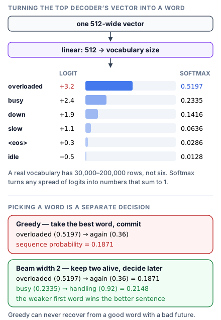
First a linear projection maps the vector to one number per vocabulary entry. Those numbers are logits — unbounded scores, positive or negative, with no interpretation as probabilities. In a real model this matrix is enormous: 4096 × 128,000 is over half a billion parameters, often the single largest matrix in the network, and frequently tied to the embedding table to avoid paying for it twice.

Then softmax turns the logits into a distribution that sums to 1. Note that it is the gaps between logits that matter, not their absolute size — adding a constant to every logit changes nothing.

Picking a word is a separate decision

Here is the distinction that most explanations blur: the model outputs a distribution, not a word. Choosing which word to emit is a decision made outside the model, and it is where the temperature and top-p knobs live.

Greedy decoding takes the highest-probability token and commits. It is deterministic, cheap, and locally shortsighted in a way that has a name.

Beam search exists because the highest-probability word does not always begin the highest-probability sentence. Keep the top k candidates alive instead of one, extend each, and rank by the total probability of the whole sequence. With k = 2 on the numbers above:

greedy   : overloaded (0.5197) → again    (0.36)  =  0.1871
beam k=2 : busy       (0.2335) → handling (0.92)  =  0.2148   ← wins

Greedy takes overloaded because 0.5197 beats 0.2335, and is then stuck with a weak continuation. Beam search keeps busy alive long enough to discover it has a much stronger one, and finishes with the better sentence despite starting from the weaker word. This is the entire argument for beam search: a locally optimal first choice can be globally worse, and greedy has no way to find out.

Two honest caveats. Sequence probability shrinks with every token, so longer candidates are penalised simply for being longer — real implementations divide by length or by some power of it. And beam search is largely not what serves modern chat models: it costs k times the compute, and optimising for the most probable sequence produces text that is noticeably bland and repetitive. It remains standard in machine translation and other tasks with one right answer, while open-ended generation uses the sampling methods below.

That distinction — the model gives you a distribution, you decide what to do with it — is what the rest of this lesson is about.

Autoregressive inference executes in two distinct phases with fundamentally different computational profiles. The prefill phase processes the entire input prompt in a single parallel forward pass, populating the KV cache. The decode phase generates output tokens one at a time, each depending on all previous tokens. These two phases hit different hardware bottlenecks — understanding which bottleneck dominates determines how you optimize serving.

Prefill (prompt processing)

The prefill phase takes the full input sequence of N tokens and runs one forward pass through the model. All N tokens are known upfront — there is no autoregressive dependency between them — so the full sequence is processed in parallel through every attention layer. The key and value projections for every token at every layer are computed and stored in the KV cache.

The computation is dominated by matrix multiplications: X @ W_Q, X @ W_K, X @ W_V, QK^T, weights @ V, and the feed-forward layers. For a 70B model processing 2048 tokens, this is approximately 2 * 70B * 2048 ≈ 287 trillion FLOPs (the factor of 2 accounts for multiply-add, and each parameter participates in one matmul per token). An A100-80GB delivers ~312 TFLOPS in FP16, so the theoretical minimum prefill time is 287T / 312T ≈ 920ms. In practice, with memory overhead and kernel inefficiencies, Llama 3 70B prefills 2048 tokens in ~100-200ms on 4×A100 (tensor-parallel across GPUs).

Prefill time determines TTFT (time to first token) — the latency a user perceives between sending a prompt and seeing the first output character. For GPT-4o via the OpenAI API, TTFT on a typical prompt is 200-500ms. For a self-hosted 70B model on 4×A100, TTFT ranges from 50ms (short prompt) to several seconds (128K context).

Prefill is compute-bound: the GPUs are fully utilized doing matrix multiplications, and the bottleneck is arithmetic throughput, not memory bandwidth.

Decode (token generation)

After prefill, the decode phase generates one token per forward pass. Each step:

• Compute Q, K, V for the single new token (one row, not N rows)
• Attend to all cached K/V from all previous tokens
• Pass through feed-forward layers
• Produce logits over the vocabulary
• Sample the next token
• Append the new K/V to the cache

The computation per decode step for a 70B model is approximately 2 * 70B ≈ 140 billion FLOPs (one token through all parameters). But the actual bottleneck is not compute — it's memory bandwidth. The model must read all 70B parameters (140GB in FP16) from GPU memory for every single output token. An A100's memory bandwidth is 2 TB/s, so reading 140GB takes ~70ms. The arithmetic (140 GFLOPS) takes only ~0.5ms at 312 TFLOPS capacity. The GPU's compute units are >99% idle during decode — they're waiting for data to arrive from memory.

This is why decode speed for large models is measured in tokens per second (TPS), typically 20-40 TPS for a 70B model on 4×A100. The A100's memory bandwidth is the ceiling. Quantization (reducing model weights from FP16 to INT4) cuts memory reads by 4x, directly increasing decode TPS by nearly 4x.

The KV cache grows with each generated token. For Llama 3 70B with GQA (8 KV heads, 128 d_head, 80 layers): each new token adds $2 \cdot 8 \cdot 128 \cdot 80 \cdot 2 \text{bytes} = 327 \text{KB}$ to the cache. At 4096 generated tokens, the KV cache is ~1.3 GB. At 128K tokens, it's ~42 GB — a significant fraction of total GPU memory.

Sampling strategies

The model's final layer produces a logit vector of shape (vocab_size,) — one score per vocabulary token. Sampling strategies convert these raw logits into a probability distribution and select a token.

import torch
import torch.nn.functional as F

def sample_token(logits, temperature=1.0, top_k=0, top_p=1.0, min_p=0.0):
    """
    logits: (vocab_size,) — raw model output for one position
    Returns: sampled token index
    """
    # Temperature scaling
    if temperature != 1.0:
        logits = logits / temperature
    
    # Top-k filtering
    if top_k > 0:
        top_k_values, _ = torch.topk(logits, top_k)
        threshold = top_k_values[-1]
        logits = torch.where(logits < threshold, torch.tensor(float('-inf')), logits)
    
    # Convert to probabilities
    probs = F.softmax(logits, dim=-1)
    
    # Min-p filtering (Nguyen et al. 2024)
    if min_p > 0.0:
        max_prob = probs.max()
        min_threshold = min_p * max_prob
        logits = torch.where(probs < min_threshold, torch.tensor(float('-inf')), logits)
        probs = F.softmax(logits, dim=-1)
    
    # Top-p (nucleus) filtering
    if top_p < 1.0:
        sorted_probs, sorted_indices = torch.sort(probs, descending=True)
        cumulative_probs = torch.cumsum(sorted_probs, dim=-1)
        # Remove tokens with cumulative probability above the threshold
        sorted_mask = cumulative_probs - sorted_probs > top_p
        sorted_probs[sorted_mask] = 0.0
        sorted_probs = sorted_probs / sorted_probs.sum()
        # Sample from filtered distribution
        sampled_idx = torch.multinomial(sorted_probs, 1)
        return sorted_indices[sampled_idx].item()
    
    # Standard sampling from the (possibly filtered) distribution
    return torch.multinomial(probs, 1).item()

Greedy decoding — temperature=0 (or equivalently, always take argmax(logits)). Deterministic, coherent, but repetitive. Used for factual tasks where you want the single most likely answer.

Temperature — divides logits by T before softmax. T=0.7 (the default for most chat models) slightly sharpens the distribution, reducing randomness while maintaining diversity. T=1.5+ produces creative but potentially incoherent text. T→0 approaches greedy.

Top-k (Fan et al. 2018) — zero out all tokens except the k most probable. k=50 is a common default. The problem: k=50 might be too restrictive when the distribution is flat (many reasonable continuations) and too permissive when it's peaked (one obvious next word plus 49 low-probability tokens).

Top-p / nucleus sampling (Holtzman et al. 2020) — keep the smallest set of tokens whose cumulative probability exceeds p. Typically p=0.9 or p=0.95. This adapts: when the model is confident, nucleus might contain 3-5 tokens; when uncertain, it might contain hundreds. This adaptivity makes top-p generally superior to fixed top-k.

Min-p (Nguyen et al. 2024) — discard any token whose probability is below min_p * max_probability. If the highest-probability token has p=0.4 and min_p=0.1, any token below 0.04 is discarded. This scales naturally with the distribution's peakedness and avoids the arbitrary fixed threshold of top-k.

Frequency/presence penalty — applied to the logits before sampling. Frequency penalty subtracts penalty * count(token) from each token's logit, where count is how many times it has appeared in the output so far. Presence penalty subtracts a fixed value for any token that has appeared at all. These reduce repetition.

Speculative decoding

Leviathan et al. (2023) and Chen et al. (2023) independently proposed speculative decoding: use a small, fast "draft" model to generate N candidate tokens, then verify all N in a single forward pass of the large "target" model.

def speculative_decode(draft_model, target_model, prompt_ids, n_speculative=5):
    """
    draft_model: small model (e.g., Llama 3 1B) — fast but lower quality
    target_model: large model (e.g., Llama 3 70B) — slow but high quality
    n_speculative: number of draft tokens to generate per verification step
    """
    generated = list(prompt_ids)
    
    while not should_stop(generated):
        # Draft phase: generate N tokens quickly with the small model
        draft_tokens = []
        draft_input = torch.tensor([generated])
        for _ in range(n_speculative):
            draft_logits = draft_model(draft_input).logits[:, -1, :]
            draft_token = torch.argmax(draft_logits, dim=-1)
            draft_tokens.append(draft_token.item())
            draft_input = torch.cat([draft_input, draft_token.unsqueeze(0).unsqueeze(0)], dim=-1)
        
        # Verify phase: run all N+1 positions through the target model in ONE pass
        verify_input = torch.tensor([generated + draft_tokens])
        target_logits = target_model(verify_input).logits  # (1, seq_len, vocab)
        
        # Accept draft tokens that match what the target model would have generated
        n_accepted = 0
        for i, draft_token in enumerate(draft_tokens):
            target_token = torch.argmax(target_logits[:, len(generated) + i - 1, :], dim=-1).item()
            if draft_token == target_token:
                generated.append(draft_token)
                n_accepted += 1
            else:
                generated.append(target_token)
                break
        
        if n_accepted == len(draft_tokens):
            # All draft tokens accepted — also take the target's next token
            bonus_token = torch.argmax(target_logits[:, -1, :], dim=-1).item()
            generated.append(bonus_token)
    
    return generated

The speedup comes from amortizing the target model's expensive forward pass across N tokens instead of 1. If the draft model's acceptance rate is 70-80% (typical when the draft model is a distilled version of the target), you get 2-3x decode speedup with mathematically identical output distribution — the verification step guarantees the final output is exactly what the target model would have produced alone.

In production: Anthropic, Google, and inference providers like Together AI and Fireworks use speculative decoding. Common draft/target pairs: Llama 3 1B / Llama 3 70B, or purpose-trained draft heads attached to the main model.

Continuous batching

Traditional static batching waits until all requests in a batch finish before starting new ones. If a batch of 8 requests has 7 short answers (50 tokens) and 1 long answer (500 tokens), the 7 finished slots sit idle for ~90% of the time.

Continuous batching (Yu et al. 2022, implemented in vLLM): when any request in the batch finishes, immediately insert a new request into that slot. The batch stays full at all times, maximizing GPU utilization. vLLM reports 2-4x throughput improvement over static batching for production workloads with variable output lengths.