Scaled dot-product attention

Do it once by hand

The formula for attention fits on one line, and that is exactly why it is hard to learn from. Before the algebra, here is the entire calculation carried out on three tokens with numbers small enough to check on paper.

The sentence is the one from the last lesson, and we are computing the new representation of it. Take three tokens — server, request, it — and give each one four dimensions. Pretend, for readability, that training has landed on dimensions that mean something: machine-ness, message-ness, subject-role, and capacity. Real models have no such labels; they just have 512 numbers whose meanings are entangled. The mechanism is identical either way.

Every token carries three vectors. Its query is what it is looking for. Its key is what it advertises to anyone looking. Its value is what it hands over when someone picks it. Here they are:

              machine  message  subject  capacity
q  "it"          1.0      0.0      0.5      1.0     ← looking for a machine that can be overloaded
k  "server"      1.0      0.0      0.8      1.0     ← advertises: machine, subject, has capacity
k  "request"     0.0      1.0      0.2      0.0     ← advertises: message
k  "it"          0.2      0.2      0.4      0.1

v  "server"      0.9      0.1      0.7      0.8
v  "request"     0.1      0.9      0.2      0.1
v  "it"          0.3      0.3      0.5      0.2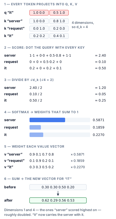

Step 1 — score every key against the query. A dot product. Multiply matching dimensions and add. For server: $1\times 1.0 + 0\times 0.0 + 0.5\times 0.8 + 1\times 1.0 = 2.40$. For request: $0 + 0 + 0.5\times 0.2 + 0 = 0.10$. For it itself: $0.2 + 0 + 0.2 + 0.1 = 0.50$. The query and the server's key agree on machine-ness and on capacity, so they score high. The request's key agrees on nothing the query asked about, so it scores near zero. That is the entire matching mechanism — no lookup table, no rule about pronouns, just whether two vectors point the same way.

Step 2 — divide by the square root of the dimension. Here $d_{k} = 4$, so divide by 2: 1.20, 0.05, 0.25. Why this is necessary rather than cosmetic is derived below; for now it is one division.

Step 3 — softmax. Exponentiate each score and divide by the total. $e^{1.20} = 3.3201$, $e^{0.05} = 1.0513$, $e^{0.25} = 1.2840$, summing to 5.6554. Divide through and the three weights are 0.5871, 0.1859, 0.2270. They sum to 1, which is the point: attention is a budget being spent, and softmax is what makes it a budget.

Step 4 — weight the value vectors and add them up. Each dimension separately:

machine :  0.5871×0.9 + 0.1859×0.1 + 0.2270×0.3  =  0.6151
message :  0.5871×0.1 + 0.1859×0.9 + 0.2270×0.3  =  0.2941
subject :  0.5871×0.7 + 0.1859×0.2 + 0.2270×0.5  =  0.5616
capacity:  0.5871×0.8 + 0.1859×0.1 + 0.2270×0.2  =  0.5337

Now compare what went in with what came out. The token "it" arrived carrying [0.3, 0.3, 0.5, 0.2] — a bland vector, because "it" means almost nothing on its own. It leaves carrying [0.62, 0.29, 0.56, 0.53]. Machine-ness roughly doubled. Capacity more than doubled. Message-ness barely moved.

That is coreference resolution, and there is no step in it that is about pronouns. The vector for "it" now carries the server, because the server won the largest share of a budget that was allocated by a dot product. Everything above this line in the lesson is a scaled-up version of exactly these four steps.

import numpy as np

K = np.array([[1.0, 0.0, 0.8, 1.0],    # server
              [0.0, 1.0, 0.2, 0.0],    # request
              [0.2, 0.2, 0.4, 0.1]])   # it
V = np.array([[0.9, 0.1, 0.7, 0.8],
              [0.1, 0.9, 0.2, 0.1],
              [0.3, 0.3, 0.5, 0.2]])
q = np.array([1.0, 0.0, 0.5, 1.0])     # query for "it"

scores = K @ q                          # [2.40, 0.10, 0.50]
scaled = scores / np.sqrt(4)            # [1.20, 0.05, 0.25]
w = np.exp(scaled) / np.exp(scaled).sum()
print(w.round(4))                       # [0.5871 0.1859 0.227 ]
print((w @ V).round(4))                 # [0.6151 0.2941 0.5616 0.5337]
print(V[2].round(4))                    # [0.3 0.3 0.5 0.2]        ← "it" before

The same thing, as one matrix multiply

Doing that per token would be hopeless at scale — a 2,000-token sequence would need four million dot products issued one at a time. The fix is not a different algorithm, only a different shape. Stack the token vectors as rows of a matrix X, and every step above becomes a single batched operation.

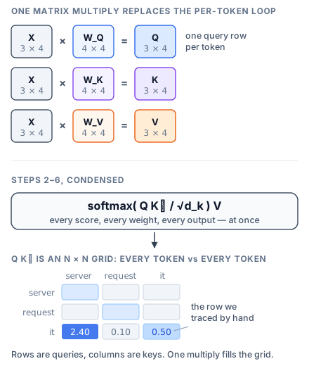
The row we just traced by hand is one row of Q Kᵀ — the row where the query is "it" and the columns are 2.40, 0.10, 0.50. The full grid holds that calculation for every token as query against every token as key. Rows are queries; columns are keys; the grid is square in the sequence length, which is where the quadratic cost comes from and why most of the rest of this course is about making that grid cheaper.

The attention function takes three inputs — queries, keys, and values — and computes a weighted sum of values where the weights are determined by the compatibility between queries and keys. The full operation is $$\text{Attention}(Q, K, V) = \text{softmax}(\frac{\text{QK}^{T}}{\sqrt{d_{k}}}) \cdot V$$. Each component has a specific computational role.

Projecting into Q, K, V

Starting from a sequence of N token representations, each a d_model-dimensional vector (stacked into a matrix X of shape (N, d_model)), the model projects into three separate spaces:

Q = X @ W_Q    # (N, d_k)
K = X @ W_K    # (N, d_k)
V = X @ W_V    # (N, d_v)

W_Q, W_K, and W_V are learned weight matrices. In the standard Transformer, $d_{k} = d_{v} = \frac{d_{\text{model}}}{H}$ where H is the number of attention heads, but the projection can target any dimension. The query vector for token i encodes "what this token is looking for." The key vector for token j encodes "what this token offers." The value vector for token j carries the actual content that will be transmitted if token j is attended to.

The query/key separation is critical. Without it — if the model used the same representation for both matching and content — the attention pattern would be constrained to a symmetric similarity metric. With separate Q and K projections, the model can learn asymmetric relationships: token A attends to token B without requiring B to attend to A. This asymmetry is essential for directional linguistic relationships: a verb should attend to its subject (to agree in number), but the subject does not need the same kind of attention to the verb. The separate value projection adds another degree of freedom: what a token advertises about itself (its key) can differ from what it transmits when attended to (its value).

Computing attention scores

The raw scores are the dot products between every query and every key:

Entry scores[i][j] is the dot product between query i and key j — a scalar measuring how much token i should attend to token j. This produces an N x N matrix where every position in the sequence is compared to every other position.

The computational cost of this matrix multiply is O(N² * d_k). For a typical configuration — N = 4096 tokens, d_k = 128 — this is $4096 \times 4096 \times 128 = ~2.1 \text{billion}$ multiply-add operations per attention head per layer. At N = 128K tokens (the context length of GPT-4, Claude, and Gemini), the score matrix alone contains $128K \times 128K = 16.4 \text{billion}$ entries per head.

The scaling factor

Before softmax, the scores are divided by sqrt(d_k). This is not cosmetic — it is numerically necessary.

Dot products between random vectors grow with the dimensionality of those vectors. If the entries of Q and K are independent random variables with mean 0 and variance 1, then each dot product q · k is a sum of d_k terms, each with variance 1. The variance of the sum is d_k, so the standard deviation of the dot products is sqrt(d_k).

At d_k = 128, dot products will typically range from about -20 to +20 (a few standard deviations). The softmax function exp(x_i) / sum(exp(x_j)) pushes most of its probability mass onto the largest value when the inputs are large in magnitude. At this scale, the softmax output is nearly one-hot: the largest score gets weight ~1.0, everything else gets ~0.0. The gradients of softmax in this saturated regime are near zero, stalling learning.

Dividing by $$\sqrt{d_{k}} = \sqrt{128} ≈ 11.3$$ rescales the dot products to have unit variance, keeping them in the range where softmax produces informative (non-saturated) gradients. Vaswani et al. (2017) noted that additive attention (Bahdanau-style) does not suffer from this problem because the tanh nonlinearity constrains the score range, but dot-product attention requires explicit scaling.

import numpy as np

d_k = 128
q = np.random.randn(d_k)
k = np.random.randn(d_k)

# Without scaling: dot product has std dev ~sqrt(128) ≈ 11.3
unscaled = q @ k
print(f"Unscaled dot product: {unscaled:.2f}")  # typically -20 to +20

# With scaling: dot product has std dev ~1
scaled = (q @ k) / np.sqrt(d_k)
print(f"Scaled dot product: {scaled:.2f}")  # typically -2 to +2

Softmax and attention weights

After scaling, softmax is applied to each row independently:

Row i of the weight matrix sums to 1 and contains the attention distribution for token i — how much it attends to each position in the sequence. The softmax ensures non-negative weights that form a valid probability distribution. A weight of 0.4 on position j means token i draws 40% of its updated representation from the value vector at position j.

Computing the output

The final step multiplies the attention weights by the value matrix:

Row i of the output is a weighted average of all value vectors, where the weights are determined by the query-key compatibility scores. Each output vector output[i] is sum_j(weight[i][j] * V[j]) — a blend of value vectors from across the entire sequence, with the blend determined by how well each key matched the query at position i.

Full implementation

Here is a complete numpy implementation with a worked example:

import numpy as np

def scaled_dot_product_attention(Q, K, V):
    """
    Q: (N, d_k) — query vectors
    K: (N, d_k) — key vectors
    V: (N, d_v) — value vectors
    Returns: output (N, d_v), weights (N, N)
    """
    d_k = K.shape[-1]

    # Step 1: compute raw scores
    scores = Q @ K.T  # (N, N)

    # Step 2: scale by sqrt(d_k)
    scores = scores / np.sqrt(d_k)

    # Step 3: softmax (row-wise, numerically stable)
    scores_max = scores.max(axis=-1, keepdims=True)
    exp_scores = np.exp(scores - scores_max)
    weights = exp_scores / exp_scores.sum(axis=-1, keepdims=True)

    # Step 4: weighted sum of values
    output = weights @ V  # (N, d_v)

    return output, weights


np.random.seed(0)
N = 5       # sequence length
d_model = 64
d_k = 64
d_v = 64

X = np.random.randn(N, d_model) * 0.1

W_Q = np.random.randn(d_model, d_k) * 0.05
W_K = np.random.randn(d_model, d_k) * 0.05
W_V = np.random.randn(d_model, d_v) * 0.05

Q = X @ W_Q  # (5, 64)
K = X @ W_K  # (5, 64)
V = X @ W_V  # (5, 64)

output, weights = scaled_dot_product_attention(Q, K, V)

print(f"Q shape: {Q.shape}")       # (5, 64)
print(f"scores shape: {(Q @ K.T).shape}")  # (5, 5)
print(f"output shape: {output.shape}")     # (5, 64)
print(f"\nAttention weights (each row sums to 1):")
for i in range(N):
    row = " ".join(f"{w:.3f}" for w in weights[i])
    print(f"  token {i}: [{row}]  sum={weights[i].sum():.4f}")

Running this produces a 5 x 5 attention weight matrix. Each row is a probability distribution showing how one token distributes its attention across all five positions. With random (untrained) weights, the distribution is roughly uniform — the structure emerges only after training. In a trained model, these distributions are typically sparse: most of the weight concentrates on 2–5 positions, with the remaining positions receiving near-zero attention. This sparsity is an emergent property of training, not an architectural constraint — the softmax can produce any distribution from uniform to one-hot.

Memory and compute costs

The attention mechanism's resource consumption is dominated by the N x N score matrix:

• Compute — The two matrix multiplications (QK^T and weights @ V) cost O(N² * d) FLOPs combined. For a single head in GPT-3 (N = 2048, d_k = 128): 2 × 2048² × 128 ≈ 1.07 billion FLOPs. With 96 heads and 96 layers: ~9.9 trillion FLOPs per forward pass just for attention (before the feed-forward layers).
• Memory — The N x N attention weight matrix must be stored for the backward pass. At N = 4096 in float32: $4096^{2} \times 4 \text{bytes} = 64 \text{MB}$ per head per layer. With 32 heads and 32 layers (Llama 3 8B): $64 \text{MB} \times 32 \times 32 = 64 \text{GB}$ — more than the model's parameters (8B × 2 bytes = 16 GB in float16). This is why FlashAttention (Dao et al. 2022) avoids materializing the full attention matrix, reducing memory from O(N²) to O(N) through tiled computation.
• Context length scaling — Doubling the sequence length quadruples both compute and memory. Going from 4K to 128K context (a 32x increase) means 1024x more attention compute and memory per head. This is the fundamental constraint that drives research into linear attention, sparse attention, and other sub-quadratic approximations.