Why attention exists
Start with a sentence you can read
Here is a sentence with a small trap in it: "The server rejected the request because it was overloaded."
What does it refer to? You answered before you finished reading — the server was overloaded, not the request. Now notice what you actually did. Nothing inside the word "it" carries that answer. Its spelling, its dictionary entry, its part of speech are all identical in the sentence "The server rejected the request because it was malformed" — where "it" flips to the request. You resolved the pronoun by looking at the other words and judging which one mattered.
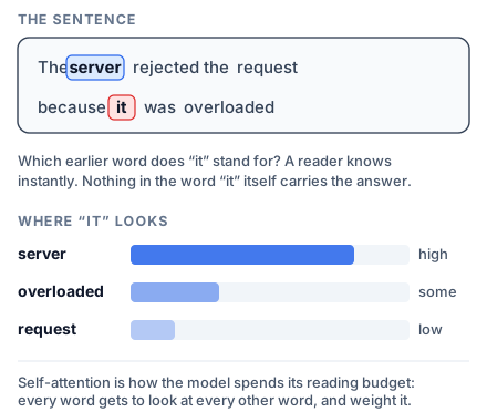
That judgment is the whole job. A model reading this sentence has to produce a representation of "it" that already knows it means the server, because everything downstream — the next layer, the next word it predicts — sees only that vector. So the question the architecture has to answer is narrow and mechanical: when building the representation of one word, how much of every other word should be mixed in?
Attention is a way of answering that with a number per pair. Every token gets a fixed budget of one unit of attention, and it distributes that budget across all the tokens it can see. Ten percent here, sixty percent there. Those numbers are computed, not stored — which means the same model handles "because it was overloaded" and "because it was malformed" without anyone writing a rule for pronouns.
Two properties of that design turn out to matter more than the linguistics. The weights are learned, so nobody enumerates what counts as relevant. And the weights are computed in parallel for every pair at once, which is what made attention worth building an architecture around rather than bolting onto an existing one.
The rest of this lesson is the road that led here: what recurrence cost, what the first attention mechanism fixed, and what remained broken until the transformer removed recurrence entirely.
What recurrence cost
A recurrent neural network processes a sequence of tokens one at a time, left to right. At each step t, it computes a new hidden state — a fixed-size vector (typically 256–1024 dimensions) that must compress everything the network has seen so far. By the time the network reaches token 200, information about token 1 has been transformed through 199 nonlinear function applications. The gradient of the loss with respect to early hidden states shrinks exponentially through repeated matrix multiplications — this is the vanishing gradient problem (Bengio et al. 1994). In practice, vanilla RNNs cannot learn dependencies longer than ~10–20 tokens.
LSTMs (Hochreiter & Schmidhuber 1997) and GRUs (Cho et al. 2014) partially solve this with gating mechanisms. An LSTM cell maintains a separate cell state c_t alongside the hidden state, with three gates (forget, input, output) that control information flow. The forget gate can learn to hold a value across many timesteps by keeping its activation near 1.0, which preserves the gradient along the cell state path. This extends effective memory to roughly 200–500 tokens in practice — enough for most sentence-level tasks, but not for multi-paragraph reasoning or document-level context. A 512-dim LSTM hidden state encoding a 1000-token document is compressing roughly 4KB of raw token IDs into 2KB of floating-point state, with the compression growing worse as the document grows. But the fundamental bottleneck remains: processing is sequential, so you cannot parallelize across sequence positions, and any information from position j that reaches position i must survive i - j sequential state updates. On GPU hardware, this means an LSTM over a 1024-token sequence requires 1024 serial steps, each waiting for the previous — the parallelism of the hardware is entirely wasted along the sequence dimension.
The encoder-decoder bottleneck
Seq2seq models (Sutskever et al. 2014) use one RNN to encode an input sequence into a single fixed-length context vector, then a second RNN to decode the output sequence from that vector. For machine translation, the encoder reads the entire source sentence and its final hidden state becomes the decoder's initial state. This final hidden state — a single vector, typically 1024 dimensions — must contain everything needed to generate the entire translation.
The compression is brutal. A 50-word source sentence might carry 200+ bits of task-relevant information (word identities, syntax, semantics, word order). A 1024-dim float32 vector stores 4096 bytes, but the effective information capacity of a learned representation is far lower. Cho et al. (2014) showed that BLEU scores on English-French translation degraded sharply for source sentences longer than ~20 words using this architecture.
Bahdanau attention — the first attention mechanism
Bahdanau, Cho, and Bengio (2014) proposed a direct fix: instead of forcing the decoder to rely on a single context vector, let it look at all encoder hidden states at every decoding step and dynamically select which ones are relevant.
The encoder is a bidirectional RNN that produces a hidden state h_j for each source position j. At each decoder step i, with decoder state s_i, the model computes an alignment score for every encoder position:
This is an additive (or "concat") score function — it concatenates (via separate linear projections) the decoder state and each encoder state, passes through tanh, then projects to a scalar. The learnable parameters are W_s, W_h (both projecting to an intermediate dimension, typically 256–512), and v (a vector that maps the intermediate representation to a single score).
The scores are normalized via softmax to produce attention weights a_{ij} = softmax(e_{ij}) over all encoder positions, and the context vector is the weighted sum .
Here is a numpy implementation of the core mechanism:
import numpy as np

def bahdanau_attention(decoder_state, encoder_states, W_s, W_h, v):
    """
    decoder_state: (hidden_dim,) — current decoder hidden state
    encoder_states: (seq_len, hidden_dim) — all encoder hidden states
    W_s: (attn_dim, hidden_dim) — projects decoder state
    W_h: (attn_dim, hidden_dim) — projects encoder states
    v: (attn_dim,) — maps to scalar score
    """
    seq_len = encoder_states.shape[0]

    # Project decoder state once: (attn_dim,)
    projected_decoder = W_s @ decoder_state

    scores = np.zeros(seq_len)
    for j in range(seq_len):
        # Project each encoder state: (attn_dim,)
        projected_encoder = W_h @ encoder_states[j]
        # Additive score: v^T * tanh(W_s * s + W_h * h_j)
        scores[j] = v @ np.tanh(projected_decoder + projected_encoder)

    # Softmax to get attention weights
    weights = np.exp(scores - scores.max())
    weights = weights / weights.sum()

    # Context vector: weighted sum of encoder states
    context = weights @ encoder_states  # (hidden_dim,)
    return context, weights


np.random.seed(42)
hidden_dim = 256
attn_dim = 128
seq_len = 10

encoder_states = np.random.randn(seq_len, hidden_dim) * 0.1
decoder_state = np.random.randn(hidden_dim) * 0.1
W_s = np.random.randn(attn_dim, hidden_dim) * 0.05
W_h = np.random.randn(attn_dim, hidden_dim) * 0.05
v = np.random.randn(attn_dim) * 0.05

context, weights = bahdanau_attention(decoder_state, encoder_states, W_s, W_h, v)
print(f"Context shape: {context.shape}")     # (256,)
print(f"Weights shape: {weights.shape}")     # (10,)
print(f"Weights sum: {weights.sum():.4f}")   # 1.0000
print(f"Max attention at position: {weights.argmax()}")
The model learns which source words to attend to for each target word. When translating "la maison bleue" to "the blue house," the decoder attending to "house" should place high weight on "maison." This was verified experimentally: Bahdanau et al. visualized the attention weight matrices and found they closely mirror word alignment tables used in statistical machine translation. The improvement was substantial — on English-French WMT'14, adding attention to the encoder-decoder model improved BLEU from ~26 (fixed context vector) to ~31 (attention), with the gain increasing as sentence length grew. For sentences of 50+ words, the attention model maintained performance while the fixed-vector baseline collapsed.
Luong attention — simpler score functions
Luong, Pham, and Manning (2015) proposed three alternative score functions that replaced Bahdanau's additive score with computationally simpler alternatives:
- Dot product — . No learnable parameters in the scoring function itself. The cheapest to compute: one dot product per encoder position.
- General — . One learnable matrix
W(hidden_dim × hidden_dim). Allows the model to learn a transformed similarity. - Concat — . Essentially Bahdanau's formulation with a single combined projection.
The dot product score became the default for subsequent work. It requires the decoder and encoder hidden states to be the same dimension, but that is the usual case.
Vaswani — attention without recurrence
Vaswani et al. (2017) "Attention Is All You Need" took the key insight — direct, learned connections between any two positions — and built an entire architecture from it. The Transformer eliminates recurrence completely. Every layer consists of a multi-head self-attention sublayer followed by a position-wise feed-forward network, with residual connections and layer normalization around each.
Two properties made this work where all previous architectures required sequential processing:
Constant path length. In an RNN, information from position j reaches position i through |i - j| sequential steps. In a Transformer, every position attends directly to every other position — the path length is 1, regardless of sequence length. Gradients flow directly between any two positions in a single backpropagation step.
Full parallelism. An RNN must compute h_1 before h_2 before h_3 — each state depends on the previous. Self-attention computes all positions simultaneously: the attention scores and outputs for every token in a sequence can be computed in a single batched matrix multiplication. On a GPU with sufficient memory, processing a 1024-token sequence takes the same wall-clock time as processing a 2-token sequence (ignoring memory bandwidth effects). This changed training throughput by orders of magnitude: the original Transformer was trained on 8 P100 GPUs for 3.5 days to achieve state-of-the-art translation quality, where comparable RNN models required weeks.
The computational tradeoff is that self-attention scales quadratically in sequence length — O(N²) attention scores versus O(N) for an RNN — but the constant factor is small (dense matrix multiplies on GPU hardware) and the parallelism advantage dominates for sequences up to tens of thousands of tokens.
The architectural trajectory
The Transformer's impact was immediate. Within two years: BERT (Devlin et al. 2018) used bidirectional self-attention for language understanding, GPT-2 (Radford et al. 2019) used causal self-attention for generation, and T5 (Raffel et al. 2019) used the full encoder-decoder architecture for sequence-to-sequence tasks. Every major language model since — GPT-4, Claude, Llama, Gemini — is a Transformer variant. The attention mechanism is the load-bearing component.