The similarity search problem

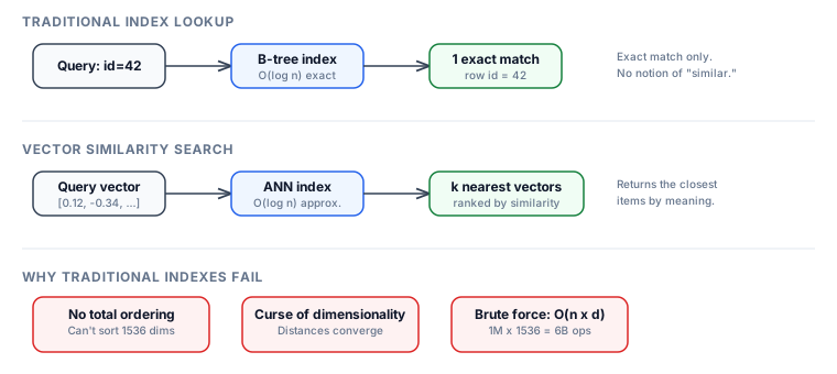
A similarity search takes a query vector and returns the k vectors in a dataset closest to it under some distance function. "Close" means geometrically nearby in the embedding space — not an exact match on any field. A text embedding model maps "how to train a neural network" and "deep learning tutorial" to points that are near each other in 768-dimensional space, even though they share almost no tokens.

Traditional databases cannot serve this workload. The rest of this lesson explains why, and what replaces them.

Why SQL indexes fail

B-tree indexes exploit total ordering: given any two keys, one is definitively less than the other. This lets a query discard half the remaining search space at each tree level, yielding O(log n) lookups.

Vectors have no total ordering. A 768-dimensional vector cannot be meaningfully sorted into a single sequence that preserves proximity in all directions simultaneously. You could index on one dimension, but neighbors in that dimension are not neighbors in the full space — the correlation between single-axis proximity and true geometric proximity drops toward zero as dimensionality increases.

Hash indexes fare no better. Locality-sensitive hashing (LSH) exists, but a standard hash index maps exact values to buckets; slight perturbations in a vector produce entirely different hashes.

What breaks concretely

B-tree range scan: Sorting 768-dimensional vectors by dimension 0 and scanning a range retrieves vectors with similar first coordinates. In a 768-dim space, this correlates almost nothing with true nearest neighbors. You would need to scan nearly the entire dataset to guarantee finding them.
Multi-column index: A composite index on (dim_0, dim_1, ..., dim_k) helps only for prefix-match queries. Nearest-neighbor search requires simultaneous proximity on all dimensions.
GIN/GiST indexes: PostgreSQL's generalized indexes support some geometric types, but their partitioning strategies degrade in high dimensions for the same reasons described below.

The curse of dimensionality

As dimensionality grows, three pathological effects compound:

Distance concentration

For uniformly distributed random vectors in d dimensions, the ratio of the farthest point's distance to the nearest point's distance converges to 1 as d increases. Beyer et al. (1999) proved that for many distributions, (dist_max - dist_min) / dist_min → 0 as d → ∞. When all points are roughly equidistant from the query, ranking by distance becomes meaningless noise.

In practice, real embeddings are not uniformly distributed — they lie on lower-dimensional manifolds. This is what makes nearest-neighbor search still useful in 768 or 1536 dimensions. But the concentration effect still tightens the distance distribution enough that naive partitioning struggles.

Volume explosion

The volume of a d-dimensional unit hypercube is 1 regardless of d, but the volume of the inscribed unit hypersphere shrinks to zero. At d = 10, the sphere occupies ~0.25% of the cube. At d = 100, it is negligible. Consequence: spatial partitioning structures (KD-trees, R-trees) that rely on bounding boxes waste almost all their enclosed volume on empty space — they cannot tightly bound the regions where points actually cluster.

Partitioning collapse

KD-trees achieve O(log n) search in low dimensions by recursively splitting along axes. In high dimensions, the query ball overlaps nearly all partitions, forcing the search to visit most branches. Empirically, KD-trees degrade to brute-force performance above ~20 dimensions (Weber et al., 1998).

Brute-force exact search

The simplest correct approach: compute the distance from the query to every vector in the dataset, then return the k smallest.

import numpy as np

def brute_force_knn(query: np.ndarray, data: np.ndarray, k: int) -> np.ndarray:
    distances = np.linalg.norm(data - query, axis=1)
    return np.argpartition(distances, k)[:k]

Complexity: O(n * d) per query, where n is the dataset size and d is the vector dimensionality.

Concrete performance:

100K vectors at 768 dims: ~50ms on a single CPU core (numpy, no BLAS threading). Acceptable for prototyping.
1M vectors at 768 dims: ~500ms per query. Too slow for real-time retrieval.
10M vectors at 1536 dims: ~10s per query. Unusable.
1B vectors at 768 dims: ~5000s per query. Absurd.

Brute-force does scale linearly with hardware — batching queries on a GPU with matrix multiplication can push 1M vectors at 768 dims to ~5ms. But this requires holding the entire dataset in GPU memory (768 dims 4 bytes 1M = 3 GB), which exhausts a single GPU's RAM by ~3B vectors at 768 dims.

The ANN tradeoff

Approximate nearest neighbor (ANN) algorithms accept a small reduction in accuracy in exchange for sublinear query time. Instead of guaranteeing the true k nearest neighbors, an ANN index returns a set that overlaps heavily with the true answer — typically 95-99% overlap for well-tuned indexes.

The core idea: build a data structure at index time that lets the query skip most of the dataset while still finding nearly all true neighbors. Different algorithms achieve this differently:

Graph-based (HNSW): Build a navigable graph; greedily traverse it toward the query.
Partition-based (IVF): Cluster vectors; search only the few clusters closest to the query.
Tree-based (Annoy): Build random projection trees; search the leaves closest to the query.
Hash-based (LSH): Hash vectors so that nearby vectors collide; search only the matching buckets.

All of these trade the same currency: more work at query time buys higher recall. The relationship is smooth and tunable — you can dial recall from 80% to 99.9% by adjusting a single parameter, paying proportionally more latency.

Recall@k: the metric that matters

Recall@k measures what fraction of the true k-nearest neighbors the approximate search actually returns:

recall@k = |ANN_result ∩ true_kNN| / k

recall@10 = 0.95 means the ANN index returned 9.5 of the 10 true nearest neighbors on average.
recall@10 = 1.0 means exact search — no approximation error.
recall@10 = 0.5 means half the results are wrong — unacceptable for most applications.

Why recall, not precision

In the k-nearest-neighbor setting, the result set size is fixed at k. The ANN search always returns exactly k vectors. Precision and recall are therefore identical: precision@k = recall@k = |ANN_result ∩ true_kNN| / k. The community uses "recall" by convention.

Typical targets

Search/retrieval (RAG, recommendations): recall@10 >= 0.95. Users tolerate occasional missing results.
Deduplication / compliance: recall@10 >= 0.99. Missing a duplicate is a compliance failure.
Exploratory similarity: recall@10 >= 0.85 may suffice when results are displayed as suggestions.

Measuring recall requires ground truth

To compute recall, you need the true k nearest neighbors (from brute-force). This means evaluation always involves running exact search on a test set. In production, you measure recall offline on a held-out sample, then deploy the tuned parameters.

From brute-force to production

The path from the five-line numpy baseline to a production vector database involves:

1. Choosing a distance metric (L2, cosine, dot product) — covered in Lesson 2.

2. Choosing an ANN algorithm (HNSW, IVF, or a combination) — covered in Lessons 3 and 4.

3. Quantizing vectors to reduce memory — covered in Lesson 5.

4. Adding metadata filtering, persistence, and replication — covered in later lessons.

Each layer adds complexity but also enables a new scale regime. The goal of this course is to make every layer legible enough that you can make informed tuning decisions rather than accepting defaults blindly.

Traditional indexed lookup vs vector similarity search

Key takeaways

Similarity search finds geometrically close vectors, not exact matches — B-trees and hash indexes cannot help because vectors have no total ordering.
The curse of dimensionality causes distances to concentrate and spatial partitions to degrade above ~20 dimensions, making tree-based indexes useless for real embeddings.
Brute-force exact search is O(n * d) per query — fast enough below 100K vectors, impractical above 1M.
ANN algorithms trade a small recall loss for orders-of-magnitude speedup by pruning the search space with graphs, clusters, trees, or hashes.
Recall@k (fraction of true k-nearest neighbors returned) is the primary accuracy metric; production systems typically target 0.95-0.99.