What Inference Engineering Is

Take one model and one GPU: an 8-billion-parameter open model on a single datacenter card. Send it one request at a time and it answers at about 147 tokens a second. Fill it with as many conversations as its memory will hold — fifty, for the workload this course follows — and each one slows to about 41 tokens a second, while the card as a whole produces 2,031. Same weights, same hardware, same hourly bill, and the cost of a token has fallen nearly fourteen-fold.

Neither number is the right one. The first wastes the card; the second may be too slow for the person waiting. Somewhere between them is an operating point that serves the most people within the latency they will tolerate, and finding that point — then moving it — is the job this course is about. Those figures are computed from a published measurement, not benchmarked by us. Lesson 5 shows the arithmetic, and the end of this lesson explains the rule every number in the course follows.

Training makes the model; inference runs it

A model has two lives. Training is the process of learning its weights from data. Inference is everything after: the weights are frozen, and the work is to run them for real requests. In the previous generation of machine learning, inference was the easy half. A fraud classifier takes one input, makes one pass through a small model and returns one number, and it will do that happily on a modest CPU.

Generative models broke that. A language model does not make one pass per request. It makes one pass per token it writes, each pass reading billions of weights, and it has to remember everything it has read so far while it does. You cannot take the weights, rent a GPU and expect the result to be fast, cheap or stable under load. The gap between "the model runs" and "the model serves" is where inference engineering lives.

One request, four stages

Follow a single request from the moment it arrives.

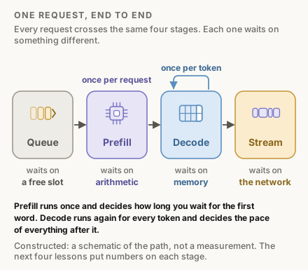
It first waits in a queue for the server to have room. Then comes prefill: the model reads the entire prompt in one pass and, as a side effect, builds a cache of what it read. Then decode: the model writes the reply one token at a time, one pass per token, consulting that cache on every pass. Finally each token is streamed back to the client as it is produced.

Two facts in that picture carry most of the course. Prefill happens once per request, and decode happens once per token. And the two are held back by different things: prefill by how fast the chip can do arithmetic, decode by how fast it can move data out of memory. Almost every technique you will meet relieves one of those two limits, and a technique that relieves the wrong one for your workload does nothing at all.

Three layers

It helps to divide the work into three layers, a framing set out in Philip Kiely's book Inference Engineering.

• Runtime — making one model on one GPU-backed machine as fast and efficient as it can be. Batching, caching, quantization, speculative decoding, and the engines that implement them.
• Infrastructure — what happens when one machine is not enough. Replicas, routing, autoscaling, cold starts, and capacity spread across regions and clouds.
• Tooling — the level of abstraction engineers are given to work at, somewhere between a black box that turns weights into an API and a bare cluster.

This course is the runtime layer: one server, made fast. The infrastructure layer is the subject of a companion course.

When it is worth doing

Most products should start on a hosted API, and many should stay there. Running your own inference earns its cost when at least one of three things is true. The API bill has become large enough that owning the hardware is cheaper. You need latency a shared endpoint cannot give you. Or you need control a vendor cannot give you — over uptime, over where data goes, over which model version answers. If none of those holds, the right amount of inference engineering is none.

How this course is built

Five layers, in the order that builds understanding, which is not the order the tools are usually listed in.

• Inference basics (lessons 1 to 5) — tokens, the forward pass, the cache, the two phases, and the clocks you will measure everything with.
• Transformer internals, just enough (6 and 7) — what the engine is actually computing.
• GPU and memory (8 to 10) — where the two limits come from.
• Optimization techniques (11 to 24) — now that you know why they work.
• Inference engines (25 to 28) — vLLM, SGLang, TensorRT-LLM and llama.cpp, which stop being black boxes once you have the first four layers.

Two lessons on other kinds of model and a capstone close it.

One service runs through all of it: Llama-3.1-8B on a single 80 GB H100, taking 8,192-token prompts and writing 256-token replies. That is the shape of a support assistant or a retrieval-augmented answer, a long prompt and a short response. Every technique is applied to that service, so you can watch the same numbers move.

One rule governs those numbers. No GPU was used to write this course, so nothing in it is our benchmark. Every figure is one of four kinds, and says which. It is computed from public model configurations and hardware spec sheets. Or it is simulated by a small step-by-step model of an engine, with its assumptions stated. Or it is cited from someone else's published measurement, with the model, hardware and workload attached. Or it is quoted from documentation. When the last line under a diagram begins with one of those words, that is what it is telling you.

You need to be able to read Python and to have called an LLM API. You do not need to know how a transformer works. Lessons 6 and 7 teach what the rest depends on, and point to The Transformer Architecture and Attention Mechanisms, from First Principles for the full derivations.