A coordinate system for meaning

Before any neural network, here is an embedding you have used your whole life.

Every colour on a screen is three numbers between 0 and 255. Pure red is (255, 0, 0). Slightly darker red is (220, 0, 0), and it sits close to pure red. Orange is (255, 165, 0) — further away, but still closer to red than blue (0, 0, 255) is. Nobody wrote down that orange resembles red. It falls out of the coordinates.

That is the entire trick. Three numbers replace an unbounded vocabulary of colour names, comparison becomes arithmetic, and similarity that you would otherwise have to hand-list is simply distance.

Latitude and longitude do the same for places. Two numbers locate anywhere on Earth, and the distance between two pairs of numbers is the distance between the two places. You do not need a table of which cities are near which.

An embedding is this idea applied to meaning: a coordinate system in which the coordinates of two things are close when the things mean similar things. The differences from RGB are that there are more than three numbers, and that nobody chooses what they measure.

Nobody chooses the axes

With colour, a human decided the axes are red, green and blue. You could imagine doing the same for meaning: axis 1 is how animal-like something is, axis 2 is how expensive, axis 3 is how dangerous. Give every word a score on each and you have a hand-built semantic space.

People tried. It does not work, for two reasons that are worth internalising because they explain why the field went the way it did.

You cannot enumerate the axes. Meaning has no finite list of independent qualities. Every new domain demands new ones, and the ones you have interact.

You cannot score consistently. Ask ten people how dangerous a ladder is, on a scale of 0 to 1, and you get ten answers. Multiply by 50,000 words and 300 axes and you have a project no organisation has ever completed.

So modern embeddings invert the problem. You do not define the axes; you define what closeness should mean, and let an optimisation procedure discover coordinates that satisfy it. You tell the model, through millions of examples, that these two sentences should end up near each other and those two should not. The model finds numbers that make it so. What each individual dimension ends up measuring is not decided in advance, is usually not nameable afterwards, and does not need to be.

This is why "which dimension means brake?" has no answer. There isn't one. Meaning is carried by direction in the whole space, not by any single coordinate.

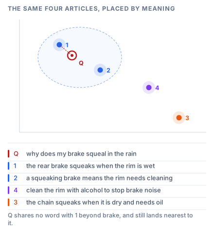
Nobody assigns the axes; training finds coordinates that put related sentences near each other and unrelated ones apart

Seeing the bike shop in two dimensions

Real embeddings have hundreds of dimensions, which nobody can picture. But the structure survives projection down to two, and that structure is what matters.

The two brake-and-rim articles sit near each other. The chain-and-oil article sits well away from them: it shares the word squeaks with D1, but shares almost nothing else, and the space is organised by meaning rather than by spelling. The rim-cleaning article sits between the brake cluster and the maintenance region, because it genuinely is between them.

Drop the customer's question into the same space and it lands inside the brake cluster, nearest D1. Not because squeal is spelled like squeaks — it isn't — but because a model that has read a great deal of English has learned that complaints about squealing, squeaking and grinding brakes occur in the same contexts, and that rain and wet do too.

Notice what just happened to the tie from Lesson 1. Word matching could not separate D1, D2 and D4, because it could see only brake. Geometry separates them easily, because it can see everything else.

Neighbourhoods, and one displacement that repeats

Zoom out from four articles to a whole vocabulary and the same structure appears at every scale: related words occupy the same region, and unrelated ones sit far apart. Nobody drew those boundaries. They are a by-product of training on text where those words kept the same company.

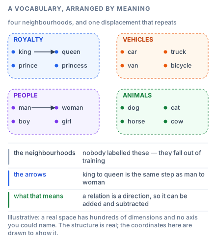
Related words occupy the same neighbourhood, and the offset from king to queen is the same offset as man to woman

The arrows are the part worth staring at. The step from king to queen is the same step, in the same direction and of the same length, as the step from man to woman. A relation — in this case something like change the gender — has become a direction in the space, and a direction is a thing you can add to any vector.

That is why the famous piece of vector arithmetic works at all: take king, subtract man, add woman, and you land next to queen. Lesson 7 covers where this comes from and how much it is oversold, but the geometric claim is the honest one to hold onto now — relations are displacements, and displacements are reusable.

Measuring closeness

Once things are points, "similar" needs a definition. There are three in common use and you should be able to compute all of them by hand.

Dot product multiplies the vectors element by element and adds the results up.

a \cdot b = \sum_{i=1}^{d} a_{i} \cdot b_{i}

Length, also called the norm, is the distance from the origin to the point.

\lVert a \rVert = \sqrt{\sum_{i=1}^{d} a_{i}^{2}}

Cosine similarity is the dot product divided by both lengths, which leaves only the angle between the two vectors.

\cos(a, b) = \frac{(a \cdot b)}{(\lVert a \rVert \cdot \lVert b \rVert)}

Two dimensions are enough to see why the choice matters. Take three vectors: a = (3, 4), b = (6, 8), c = (−4, 3).

text

a·b = 50   |a| = 5   |b| = 10   cos = 1.0000   L2 distance = 5.0000
a·c =  0   |a| = 5   |c| =  5   cos = 0.0000   L2 distance = 7.0711
b·c =  0   |b| = 10  |c| =  5   cos = 0.0000   L2 distance = 11.1803

a and b point in exactly the same direction — b is just a doubled — so their cosine is 1, a perfect match. Their dot product is 50 and their straight-line distance is 5, neither of which says "identical". That is the whole difference between the measures: cosine asks which way does it point, dot product asks which way and how far, and Euclidean distance asks how far apart are the tips.

For text, direction is usually what you want. A vector's length tends to pick up things like how long the passage was and how common its words are, which are not what you are searching on. Two articles about wet brakes should match whether one is nine words and the other is nine hundred.

The identity that makes the choice mostly moot

Most embedding models return normalized vectors, meaning every vector has been scaled to length exactly 1. Once that is true, three convenient things happen at once.

The dot product becomes the cosine, because you are dividing by 1 twice. And Euclidean distance becomes a fixed function of the cosine:

\text{L2}(a, b)^{2} = 2 \cdot (1 - \cos(a, b))

Check it on the corners:

text

cos =  1.0  ->  L2 = sqrt(2(1 - 1.0))  = 0.0000     identical
cos =  0.8  ->  L2 = sqrt(2(1 - 0.8))  = 0.6325
cos =  0.0  ->  L2 = sqrt(2(1 - 0.0))  = 1.4142     unrelated
cos = -1.0  ->  L2 = sqrt(2(1 + 1.0))  = 2.0000     opposite

Because that relationship is strictly decreasing, ranking by cosine and ranking by Euclidean distance give the identical order. For normalized vectors the choice of metric changes the numbers you print and never changes which result comes first.

The trap is assuming normalization when it isn't there. A model that returns unnormalized vectors, searched with a dot-product index, will systematically prefer long documents, because length inflates the score. Our Vector Databases, Inside and Out track works through that failure and the index configurations that cause it; for this course, the rule is simply to normalize and stop thinking about it.

What cosine similarity does not mean

Three cautions, all of which cost people time.

It is not a probability. A cosine of 0.82 does not mean 82% confidence, or an 82% chance of relevance. It is an angle, and the only thing you can do with it is compare it to another angle from the same model.

It is not comparable across models. One model may score unrelated sentences around 0.1 and another around 0.7, and neither is wrong — they have different spreads. A threshold of 0.75 tuned on one model is meaningless on the next. Lesson 9 shows how one very famous model came to score everything around 0.9.

It is not symmetric in the way you might hope. "Is this document relevant to this query?" and "is this query relevant to this document?" are different questions, and one number answers neither of them on its own. Lesson 13 covers the asymmetric encoding modern models use to handle this properly.

← Previous